Platform

Meridian

Experimental design and materials structure

Structural analysis that distinguishes required, allowed, and undetermined.

Meridian is the core MatSpace platform for planning synthesis workflows with physics bound 3D models and processing raw structural datasets. From raw powder XRD patterns and spectroscopic curves to microstructural images, Meridian treats every dataset as a physically constrained model rather than an unconstrained curve-fitting problem.

Most groups still split this work across a notebook, a vendor GUI, a desktop suite from the 1990s, and a spreadsheet that nobody else can reopen. The cost is not licence fees. It is an afternoon spent reconstructing a model that already has a name, a Rietveld job that converges on a lattice the sample cannot be, or a third Gaussian parked under a defect band because the residual looked quieter. Meridian was written for the other half of the job: knowing when a component is required, when it is merely allowed, and when the data cannot tell.

Meridian

CurveFit Lab

Named physical models, locked parameters, and a residual inspected as data.

CurveFit Lab is a fitting laboratory built around the equation. The model is a first-class object - a named expression from a materials catalogue, or one the user writes. Parameters that must stay fixed can be locked. Derived quantities are evaluated from the fit. The residual is shown next to the overlay because a high R² can still belong to the wrong model.

  • Materials equation library covering magnetic, magnetocaloric, dielectric, luminescence, and kinetic models
  • Native constraints: lock Ms, θ, a literature baseline, or a known peak centre; the remaining parameters float under Levenberg–Marquardt
  • Derived quantities (FWHM, μeff, half-life) update with the fit rather than in a separate spreadsheet
  • R², RMSE, reduced χ², per-parameter errors, and a residual panel flagged when the residual is structured
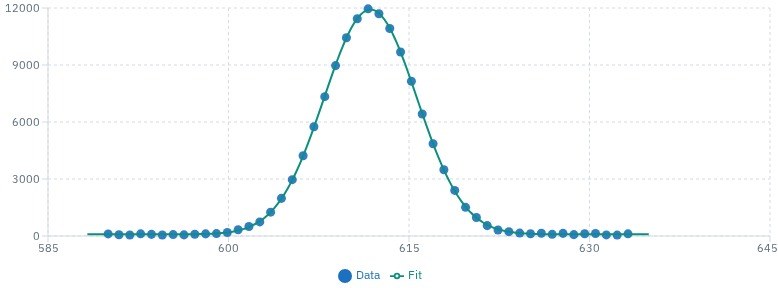
Eu³⁺ photoluminescence peak from the CurveFit demonstration. A Gaussian on a constant baseline; data and fit overlay. FWHM and area are derived from the fitted parameters, not typed in afterwards.

Warp

Virtual laboratory for designing and optimizing the experiments

Warp embeds domain-specific physical rules directly into the workspace geometry-automatically refusing invalid operations such as joint size mismatches, ground glass fittings, overfilled hydrothermal vessels, unbalanced centrifuge loads, or unsealed thermal processing environments.

Every virtual run processes experimental parameters through strict conservation algorithms:

sampleout = F(samplein, vars, tproc)

Reactions, phase transformations, and mass balance are governed by listed thermodynamic conversion pathways and kinetic models rather than unconstrained generative text. F is the first-principles calculation function that Warp employs and writes sample state on a successful run, ledger is the notebook that feeds variable to F, AI reads F function to give opinion on your virtual experiment. So, Warp ensures that stoichiometric limits, precipitation kinetics, and process time parameters remain fully conserved and reproducible.

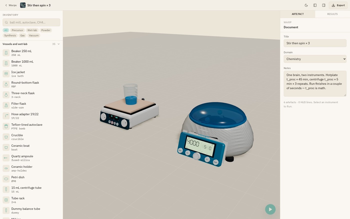
    Stir then spin × 3 on the Warp canvas. Stirrer, vessels, centrifuge, ovens, mill and furnaces seated in one protocol; samples move only along the pour graph.

    DiffractrumX

    From a pattern file to a fitted CIF without an installer, a .pcr dialect, or a server that keeps the run.

    DiffractrumX is a single web laboratory that already knows the physics of a Rietveld fit — structure factors, Caglioti widths, Thompson–Cox–Hastings pseudo-Voigt, Kα₂, Lorentz and polarisation for X-rays, Sears bound coherent lengths for neutrons — and wraps that engine in a staged instrument a materials scientist can drive in a few minutes. It does not replace an expert FullProf job on a twelve-phase mineral. It does replace the afternoon it takes to get a clean two-phase ceramic onto a CIF.

    • Forward model from real structures; demos generated from quartz, corundum, rutile and anatase, then recovered
    • One lab, two probes: laboratory X-ray (Cu, Co, Mo, Cr, Fe, Ag, custom λ, Kα₂) and constant-wavelength neutron
    • Constrained Rietveld with staged parameter release; live Rwp, χ² and GoF on the plot
    • Peak extraction, indexing, Le Bail, and a composition-constrained ab initio path when the cell is unknown
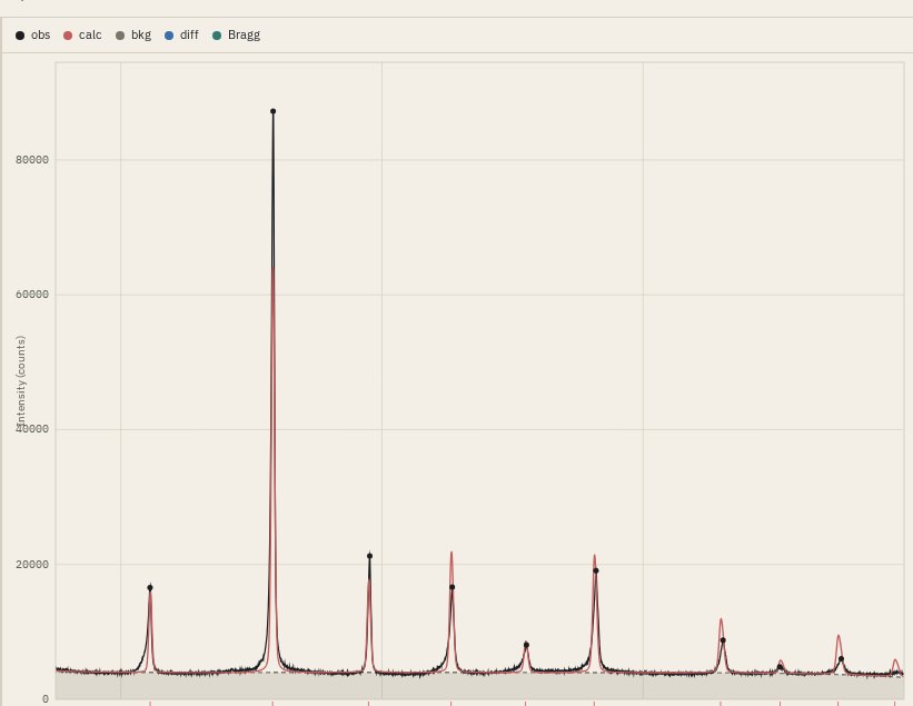
    BaTiO₃ (Pm-3m) powder pattern from the DiffractrumX demonstration. Observed counts and the calculated profile on Cu Kα, Bragg ticks under the trace. Rwp, χ² and GoF live on the same page as the plot.

    NanoImpulse

    Efficient micrographs processing to visualize materials insights with high precision.

    NanoImpulse is a local TEM, STM, SEM, EDS/Raman maps and general micrographs analysis desk for real-space images, with additional powerful tools for diffraction patterns, and core-loss EELS spectra.

    A SAED pattern is measured in the pattern, not by taking its FFT. Spots are picked from local intensity maxima, with an optional Friedel pair snapped to a real peak. Rings come from the radial profile, with a dark beam-stop excluded from the average. d-spacings stay blank until a reciprocal scale is set, either from a known d or from a real-space scale that supplies Δk (1/nm per pixel) and the camera constant Lλ in px·nm. Two chosen g vectors are used to index a zone against a cell loaded from a CIF. That cell is a trial lattice. It is not a phase identification, and no kV or camera constant is filled in if you did not enter it.

    For core-loss EELS the spectrum is a power-law fit on the pre-edge window, subtracted under the signal window you set. A structured residual is reported as a bad background, not as an element. No k-factor and no edge assignment are inferred from the energy window.

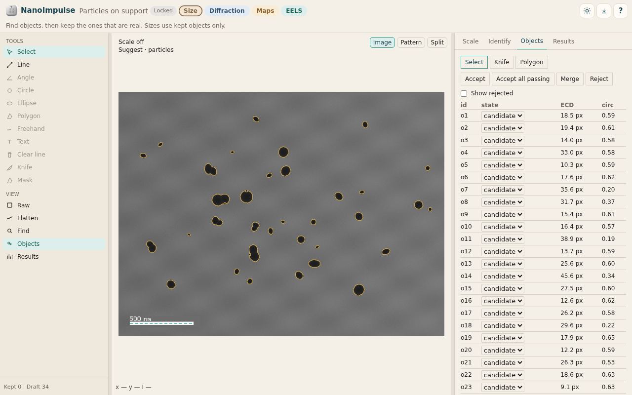
    Particles on support. Particle and grain finding is only a candidate list: sizes, aspect ratios, and nearest-neighbour distances are computed from the objects you keep, not from every segmented region.

    Spectrum Desk

    Fit peaks the physics allows. Rank the alternatives. Leave assignments unwritten when the spectrum cannot support it.

    Spectrum Desk adds a component only when the lineshape is still physical and a simpler model is not the better description. XPS requires typed doublets, charge referencing, Tougaard backgrounds, and Scofield atomic percentages. Raman defaults to a Lorentzian and does not identify a phase. Photoluminescence treats an Urbach tail as its own component, not as a stack of Gaussians. Thermoluminescence uses Kitis glow-curve deconvolution with E and s gated. Candidate models k, k+1, and k+2 are ranked by BIC. Library matches are reported as “consistent with.” The word assigned is not written from a peak list.

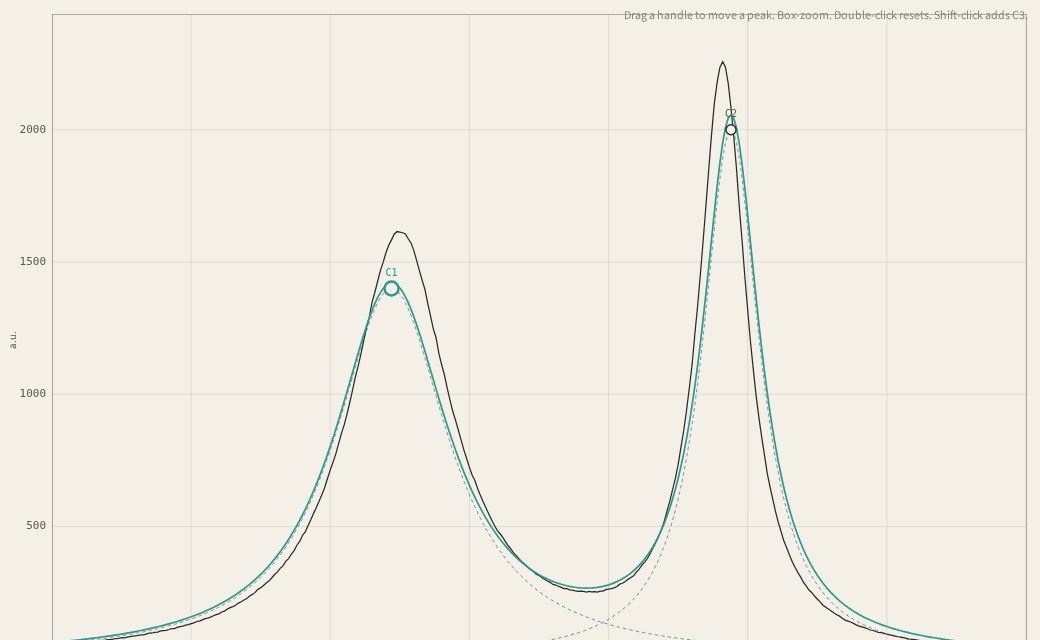
      Raman carbon D/G demonstration in Spectrum Desk — the graphene fingerprint. Two Lorentzians on the D and G bands; numbered peaks stay numbered.

      CurveFit Lab

      Named physical models, locked parameters, and a residual inspected as data.

      CurveFit Lab is a fitting laboratory built around the equation. The model is a first-class object - a named expression from a materials catalogue, or one the user writes. Parameters that must stay fixed can be locked. Derived quantities are evaluated from the fit. The residual is shown next to the overlay because a high R² can still belong to the wrong model.

      • Materials equation library covering magnetic, magnetocaloric, dielectric, luminescence, and kinetic models
      • Native constraints: lock Ms, θ, a literature baseline, or a known peak centre; the remaining parameters float under Levenberg–Marquardt
      • Derived quantities (FWHM, μeff, half-life) update with the fit rather than in a separate spreadsheet
      • R², RMSE, reduced χ², per-parameter errors, and a residual panel flagged when the residual is structured
      Eu³⁺ photoluminescence peak from the CurveFit demonstration. A Gaussian on a constant baseline; data and fit overlay. FWHM and area are derived from the fitted parameters, not typed in afterwards.

      Warp

      Virtual laboratory for designing and optimizing the experiments

      Warp embeds domain-specific physical rules directly into the workspace geometry-automatically refusing invalid operations such as joint size mismatches, ground glass fittings, overfilled hydrothermal vessels, unbalanced centrifuge loads, or unsealed thermal processing environments.

      Every virtual run processes experimental parameters through strict conservation algorithms:

      sampleout = F(samplein, vars, tproc)

      Reactions, phase transformations, and mass balance are governed by listed thermodynamic conversion pathways and kinetic models rather than unconstrained generative text. F is the first-principles calculation function that Warp employs and writes sample state on a successful run, ledger is the notebook that feeds variable to F, AI reads F function to give opinion on your virtual experiment. So, Warp ensures that stoichiometric limits, precipitation kinetics, and process time parameters remain fully conserved and reproducible.

        Stir then spin × 3 on the Warp canvas. Stirrer, vessels, centrifuge, ovens, mill and furnaces seated in one protocol; samples move only along the pour graph.

        On this platform

        Laboratories