CurveFit Lab

Live

Equation-First Nonlinear Regression for Experimental Datasets

Named physical models, locked parameters, and a residual inspected as data.

Most analysis software was built for general plotting. Origin, Igor, and Excel will draw a line through points. A Jupyter notebook will do the same if enough code is written. Those tools optimise for generality: named models, constraints, and derived quantities end up scattered across menus, licences, and local habit.

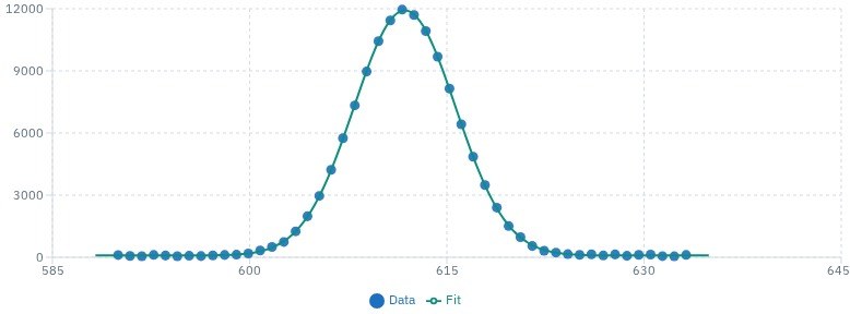
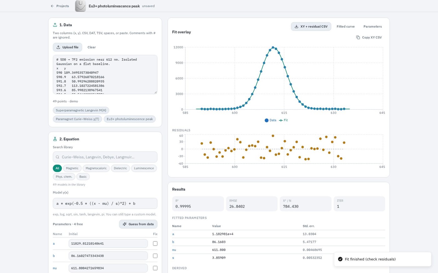
CurveFit Lab is a fitting laboratory built around the equation. The model is a first-class object - a named expression from a materials catalogue, or one the user writes. Parameters that must stay fixed can be locked. Derived quantities are evaluated from the fit. The residual is shown next to the overlay because a high R² can still belong to the wrong model.

Eu³⁺ photoluminescence peak from the CurveFit demonstration. A Gaussian on a constant baseline; data and fit overlay. FWHM and area are derived from the fitted parameters, not typed in afterwards.

Residual of the same Eu³⁺ PL fit. Structure here is treated as a warning, not as a licence to add another term.

CurveFit Lab on the Eu³⁺ demonstration: named model, four free parameters, residual panel, and derived FWHM living next to the overlay.

What it does

Materials equation library covering magnetic, magnetocaloric, dielectric, luminescence, and kinetic models
Native constraints: lock Ms, θ, a literature baseline, or a known peak centre; the remaining parameters float under Levenberg–Marquardt
Derived quantities (FWHM, μeff, half-life) update with the fit rather than in a separate spreadsheet
R², RMSE, reduced χ², per-parameter errors, and a residual panel flagged when the residual is structured
Optional AI note on physical plausibility (Analyze fit); it cannot invent or rewrite fitted numbers
Export of the measured, fitted, and residual series as CSV